AI Agents Need a Lakehouse Too
AI agents are at their most useful when they can work with a company’s own data. For that, the information they rely on has to be right. A manufacturing example shows what this means in practice for the data model, the pipelines, and the agent itself.


In this article
Ask an AI agent how often a machine stopped last year and you expect a number you can rely on. Whether the agent counted the same stoppage three times is not something the number will tell you. The answer sounds equally convincing either way.
This kind of error is most likely when an agent works directly on uncurated raw data. The same incident shows up in several systems, names differ from one system to the next, and the relationships between records are nowhere documented. Anyone who wants to make enterprise data usable for AI agents therefore has to decide up front what the data means and how the pieces fit together. A data model in a data lakehouse is where those decisions live. It ensures that the same question gives the same answer whenever it is asked, and that every figure can be traced back to its source.
This article uses a concrete example to show how such an architecture can be implemented: from the source systems through data preparation to the agent’s answer, including the data model, the rules, and the tooling involved.
Example: Analyzing machine stoppages
“Which faults caused the most stoppages last year, broken down by production line and machine type?” For an operations manager, that is an obvious question to ask. The answer helps decide which equipment the maintenance team should look at more closely.
Consider a fictional supplier of precision metal components with two plants. The information needed is already there: in the ERP system, in machine logs, and in maintenance reports. An agent is given access to these sources and asked to answer the question.
Every stoppage produces a record in three systems. The machine controller reports a fault, the shift supervisor logs a stoppage, and the maintenance team writes a report. Each record is correct on its own. If the agent counts them as three separate stoppages, its statistics are wrong.
The agent might recognize that the records belong together. It might also treat the maintenance report as a separate event. A well-formulated answer does not reveal which interpretation it chose. For a metric that the business uses to make decisions, that is not good enough.
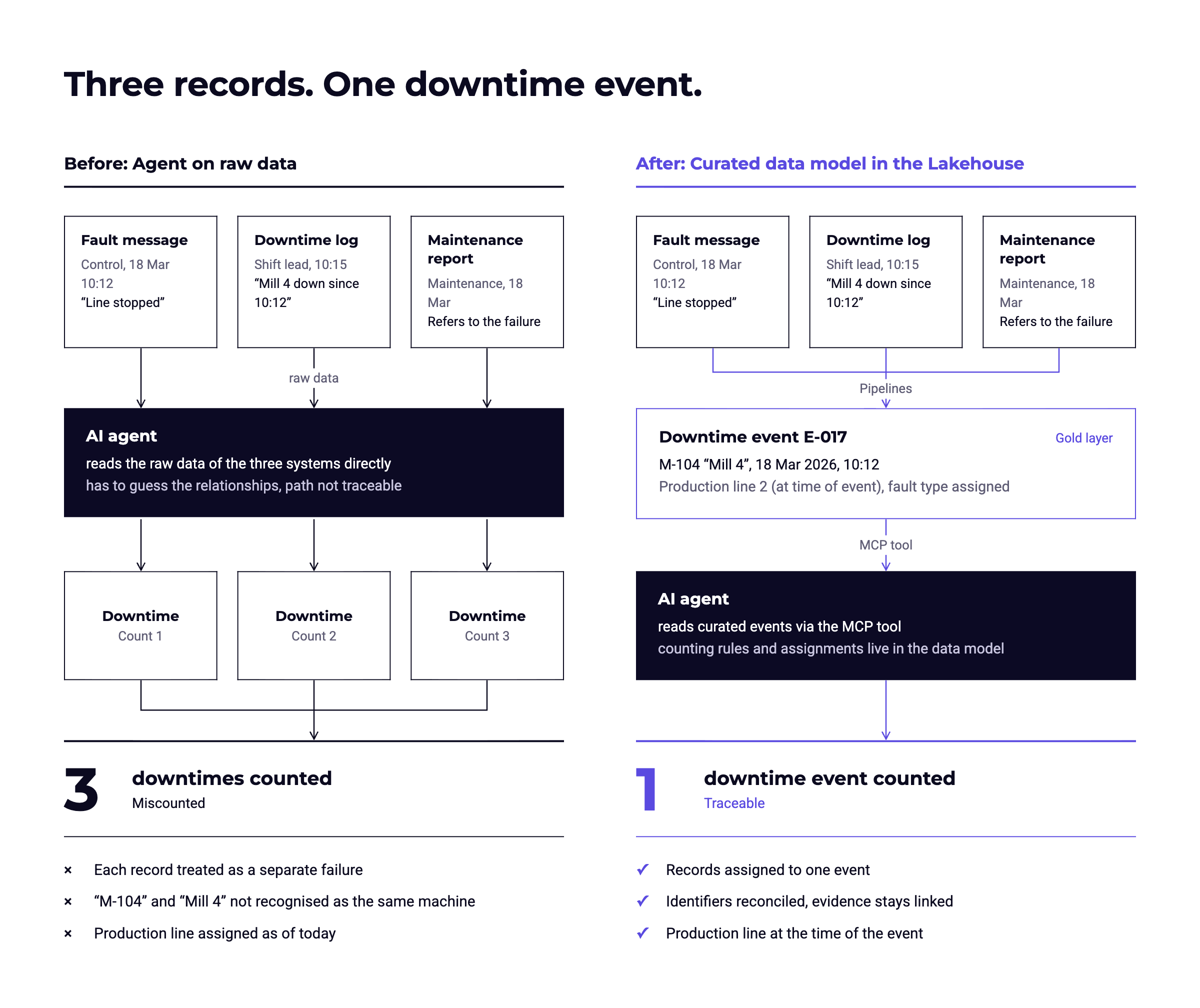
Relationships like these need to be modeled before any analysis takes place. The agent then works with a clear, traceable definition of “stoppage” instead of having to guess it anew with every request.
How data is prepared in the lakehouse
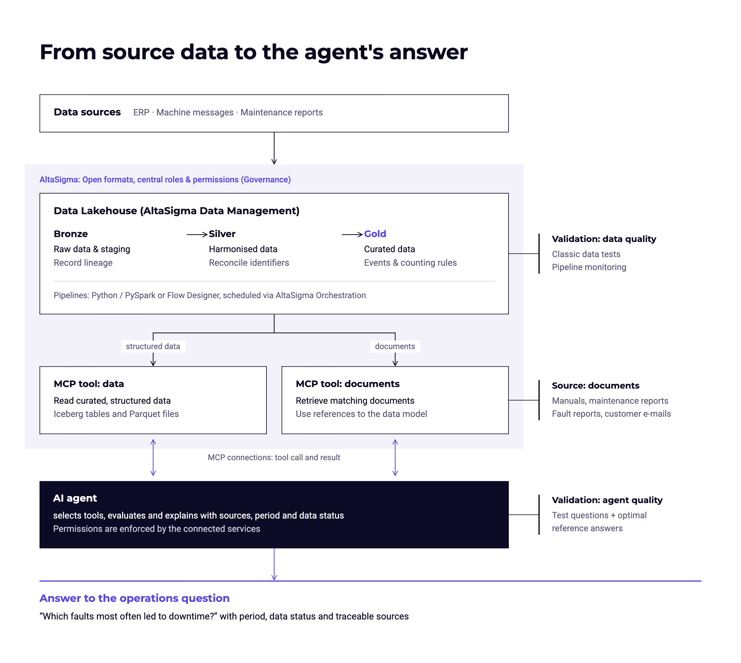
A data lakehouse brings data from different sources together and prepares it for analysis. The original records are kept. Alongside them, cleaned and business-modeled datasets are built for applications to use.
The usual way to organize this is in bronze, silver, and gold layers. What matters is the logic and rules defined between them for processing the data. Domain experts and the data team work those rules out together. They are implemented in pipelines that move data from one layer to the next. Datasets in all three layers can be managed in AltaSigma Data Management.
Bronze: Ingest the data and keep track of where it came from
At our supplier, asset records are pulled from the ERP system on a schedule, machine events arrive continuously, and maintenance reports come in as documents. Data Management provides adapters for the usual types of source, whether batch, file transfer, or streaming. The platform page on Data Management and Data Engineering gives an overview.
In the bronze layer, data stays largely in its original form. For every record, the pipeline captures which system it came from and when it arrived. That makes it possible to trace later which records an analysis was based on.
Provenance information is also relevant for corrections. If a processing rule has handled certain records incorrectly, the corrected rule can simply be rerun on the original data. There is no need for a fresh export from the source system.
Silver: Recognize the same machine across different sources
The first job in the silver layer is to identify the same machine across several sources. In the ERP system an asset is called “M-104”, in the maintenance report “Mill 4”, and in the controller perhaps just “Station 4/2”. The result of this work is a mapping table:
| machine_id | source | name_in_source | valid_from | valid_to |
|---|---|---|---|---|
| M-104 | ERP | M-104 | 2019-01-01 | – |
| M-104 | Maintenance | Mill 4 | 2019-01-01 | – |
| M-104 | Controller | Station 4/2 | 2024-06-01 | – |
When a mapping is unclear, confirming it with operations staff is more reliable than inferring it from similar-sounding names. Cases that cannot be resolved remain flagged as unresolved and do not enter the metric unnoticed.
While matching records, the pipeline also standardizes timestamps and detects records that were delivered more than once. One distinction is important here: a fault message that was accidentally imported twice is not the same thing as a maintenance report about the same fault. The report carries additional information and is kept as a separate piece of evidence.
Information from free text can be brought in as well. A language model can extract the machine reference or the action taken from a maintenance report. Those details are checked before they are used, just like data from any other source.
These pipelines can be developed in AltaSigma with Python or PySpark, or built visually in the Flow Designer.
Gold: Turn records into downtime events that can be analyzed
The gold layer answers the operational question. Each downtime event describes the machine affected, the time period, the fault type, and the production line the machine belonged to at the time of the event:
| Column | Content |
|---|---|
| event_id | unique identifier, e.g. E-017 |
| machine_id | from the mapping table |
| line_id | production line at the time of the event |
| start, end | from the earliest and latest linked record |
| fault_type | from the controller code or maintenance report |
| sources | references to the fault message, log entry, and report in bronze |
Business rules define which records belong to one event. At our supplier, the rule goes roughly like this: a fault message from the controller opens an event. A stoppage logged for the same machine that begins within 30 minutes of it belongs to that event. A maintenance report belongs to it if it names the same machine and its date falls within the event’s time window. Timing alone is not enough, because two messages in quick succession can describe different faults. That is why the documented sequence of events counts as well.
The analysis also needs the right production line. If a machine changed lines during the year, an earlier stoppage has to be assigned to the line it was on at the time. The model therefore stores the machine-to-line assignment with a validity period, just like the mapping table above. Assigning by the machine’s current location would distort the result.
What counts as a stoppage is up to the business. Does planned maintenance count? How long does an interruption have to last? Is the question about the most frequent faults, or about the ones that cost the most time in total? A frequent fault can cost less production time than a single long outage. The original question is about frequency. Ranking by duration would answer a different question. These decisions are stored as a metric definition alongside the gold table, so that everyone who uses the table works from the same definition: the agent, BI reports, and the data team.
The result is a data model in which the stoppage that was recorded three times can be analyzed as one event. The underlying records remain linked. Domain experts can check why an event was counted and why it was assigned to a particular machine or line.
Operating the pipelines
The pipelines apply the same rules to new data as it arrives. AltaSigma Orchestration runs the jobs on a fixed schedule, for example to refresh asset records at regular intervals. Streaming sources deliver continuously. How current the analysis needs to be sets the pace: a review of last year has different requirements from the question of which machines are stopped right now. Job orchestration is part of the AltaSigma platform.
The agent helps build the pipelines
AI agents do not have to wait until the data is fully prepared before they come into play. Given the source schema, the target model, and the agreed business rules, an agent can draft the PySpark code for a pipeline and suggest suitable data tests, for instance a test that ensures no event is created without a valid line assignment.
The difference from an agent working on raw data lies in when the logic is created and who reviews it. The generated code is read, tested, and approved by the data team. From then on it runs deterministically and the same way for every request. The agent that later answers operational questions reads the result instead of having to work out and execute the logic on every request.
How the agent answers the question
The agent accesses the prepared datasets through MCP tools. The Model Context Protocol, or MCP, defines the interface an agent uses to call tools. The initial access path is a generic tool: it takes a SQL query and runs it against the gold tables, which are stored as Iceberg tables or Parquet files. To write the right query, the agent first reads the table description and the metric definition stored with it. For the stoppage question, this results in the following query:
-- Metric definition from the table metadata:
-- unplanned interruptions of 5 minutes or more, planned maintenance excluded

SELECT e.line_id, m.machine_type, e.fault_type, COUNT(*) AS event_count
FROM gold.downtime_event e
JOIN gold.machine m ON m.machine_id = e.machine_id
WHERE e.start >= DATE '2025-01-01' AND e.start < DATE '2026-01-01'
  AND e.fault_type <> 'Planned maintenance'
  AND e.end - e.start >= INTERVAL '5' MINUTE
GROUP BY e.line_id, m.machine_type, e.fault_type
ORDER BY event_count DESC;
The pipeline has already consolidated the individual records into events. The agent queries what is already in the data model. It takes the counting rules from the metric definition stored with the table, not from the prompt. It still has to translate the period, filters, and grouping from the question into the query correctly and interpret the result. We will come back to that when we get to testing.
For questions that come up often, or where the query is easy to get wrong, a dedicated MCP tool can be added, for example count_downtime_events with period and grouping as parameters. The metric definition is then fixed inside the tool, and the agent no longer has to write the query itself. Whether such a tool is needed can be determined from the evaluation results in production.
If the answer should also explain what lies behind a recorded fault, other MCP tools come into play. They retrieve documents and their links to the data model, such as the maintenance report for the affected machine or the right version of the manual. Retrieving information as the basis for a generated answer is known as retrieval-augmented generation (RAG). The structured analysis provides the stoppage counts. The documents add context on fault symptoms and the actions taken. A matching passage in a manual does not, by itself, prove the cause of a specific failure.
An answer the operations manager can act on states the period, the data currency, and the sources. In this example:
The article on AI agents for handling customer inquiries shows how knowledge from tickets and documents can be made available in a similar way.
How do you know the answer is right?
Data quality and the agent’s answers can be tested separately.
At the data level, data tests and pipeline monitoring are used. Tests catch missing machine identifiers or contradictory timestamps. Known cases make it possible to check whether the business rules work: does the stoppage from March 18 that was recorded three times count exactly once? Is the historical line assignment preserved? These tests remain useful when a source or a calculation changes later. Monitoring shows whether an expected delivery failed to arrive or a pipeline did not run as planned.
At the agent level, evaluation suites with test questions and reference answers do the quality checking. A test case comprises the question, the expected answer, and the requirements for its content:
After changes to the data, the tools, or the agent configuration, the same questions can be run again and the results compared.
Cases with missing information warrant separate attention. If a shift’s records are missing, the result must not look like a shift without any faults. The agent should point out the limitation. Correct data alone does not guarantee a correct answer. That is why both levels of testing are needed.
Running the system also requires clear responsibilities and access controls. It has to be settled who maintains machine mappings, who may change metric definitions, and who is allowed to see which data. The connected services enforce those permissions when the agent retrieves data or searches documents.
Start with one production line
A first project does not have to model the whole company. For our supplier, one production line and the question of which faults cause the most stoppages there is sufficient as a starting point. Existing asset records, data platforms, and BI metrics that have already been agreed are the foundation.
The business and the data team agree on what a correct answer looks like. The data team checks the sources and implements the mappings and calculations. In the end, it has to be demonstrable that the agent counts the stoppage recorded in several systems once, assigns it to the right line, and backs up its figures. That is a better measure of progress than a single convincing demo answer.
How much effort the first step takes depends mostly on the data available and on how well operational knowledge has been documented. Missing mappings have to be resolved. Definitions that already work can be reused. More lines and more questions follow once the first scope works.
The prepared data is then available to other applications as well. BI reports use the same metric definitions. Machine learning may need more detailed measurements and events depending on the task, but it benefits just as much from resolved mappings and tested data.